Editor note: Here’s a link if you’re looking for instructions on adding a watermark to the latest version of Excel.
How to Watermark Worksheet in Excel 2010
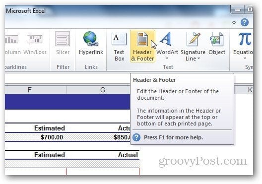
Open the worksheet on which you want to add a watermark, click the Insert tab from the Ribbon. then Header and Footer.
Under Header and Footer tools, select Design and click on Picture from Header and Footer elements.
Browse the image you want to use as your watermark. Note that after you add the picture in the header field, it will show you &[Picture] in the tab but don’t worry. Clicking on any other cell will change this text back to the image. If you want to make it appear in the middle of the sheet, just hit enter before the &[Picture] like and move it to the place where you want to header to appear.
Using WordArt as Watermark in Excel 2010
You can also use WordArt as a watermark on your Excel 2010. Click on Insert » WordArt. Select the format you want to use and type the text.
From the small text editor shortcut that appears, you can change the size of the font you want to use.
But using this WordArt may make it difficult for the user to read the worksheet. Click on Format under Design Tools.
Click on the small arrow under WordArt styles to open WordArt options.
From there, select Text Fill from the sidebar and select Solid Fill. From here, also adjust the transparency to something suitable and click Ok. This way, we can change the visibility of the watermark so that it does not cover the text in the worksheet.
Now go to Text Outline and select no line.
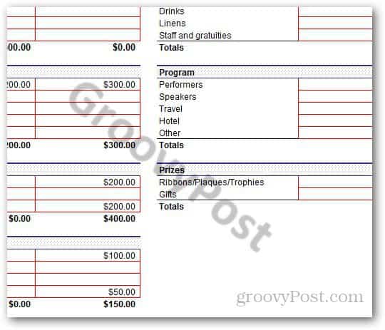
Here is how the WordArt watermark looks like. You can play around with the settings to get the result you want.
How to Add Watermark in Excel 2013
Most of the steps are the same for Excel 2013 as they are in Excel 2010. The major difference is in the layout of Excel. Just go to Insert » Header and Footer.
Click the Picture button from Header and Footer Elements.
In Excel 2013, you can use images from your computer and Office.com clip art or even search images from Bing search results and use the image as a watermark.
Using WordArt as Watermark in Excel 2013
In the start, you may find it difficult to find the WordArt option in Excel 2013 but it’s still present in the same tab as it is in Excel 2010. Go to Insert and under the Text tab, click on the WordArt icon as shown below and select what you want.
Click on the same arrow under WordArt styles to open the Format option.
A new sidebar will appear. From there, click on Text options and open Text Fill and Outline options.
Select Solid Fill under Text Fill and No line under Text Outline. Select the transparency to whatever you want and close the menu.
And you are done.
Customizing Image Watermark
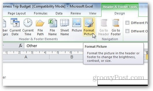
You can even customize the appearance of the picture. From the Design tab, click on Format Picture.
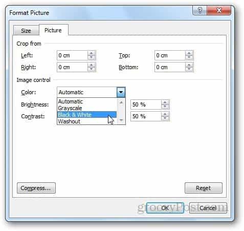
From here, you can change the size and appearance of the image. Click the Picture tab and select the settings according to your own preferences. I suggest using the Washout feature from the dropdown menu under Image Control as it makes the watermark fade out and it becomes easier for the user to read the content in the worksheet.
The compress option allows users to change the resolution and size of the picture. If you cropped out any part of the watermark from settings, you can use the compress option to delete cropped areas or even just compress the image for easy use.
However, do note that compressing the image may reduce the quality of the watermark. If you are fine with it, click Apply otherwise leave it as it is.
The steps to customize the watermark are the same for both Excel 2010 and Excel 2013.
Maybe you need to edit the dates??? How I would like to remove my initial hd as a water mark printing. Thanks HD Comment Name * Email *
Δ Save my name and email and send me emails as new comments are made to this post.
![]()

