Today I’ll show you how to create a drop-down list in a cell using Data Validation. Although I’m taking the screenshots using Excel 2016, the steps are the same if you’re using older versions. The steps are also the same in modern versions of Excel in the Microsoft 365 (formerly O365) suite.
Create a Data Table and the List of Options
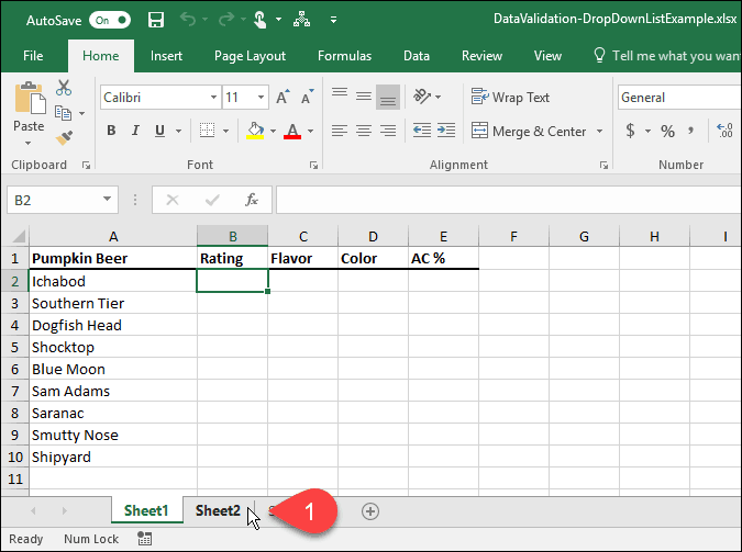
First, set up a basic data table. You can either type your data in manually or copy and paste it from another source. Next, we’re going to enter a list of options for the drop-down list. You can do that when you define the data validation or define a list in another location on the same worksheet or another worksheet. For this example, we’re going to list the options for the drop-down list on another worksheet so click one of the worksheet tabs at the bottom of the Excel window.
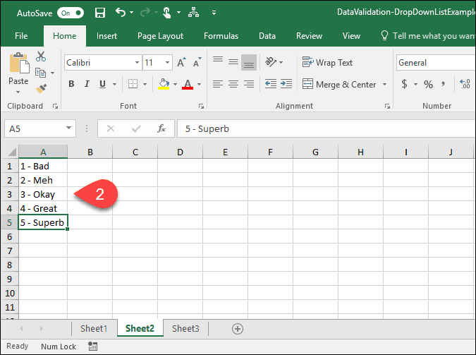
Enter each option in a column (or row), one option to a cell. Then, go back to the worksheet with your data.
Turn on Data Validation for Selected Cells
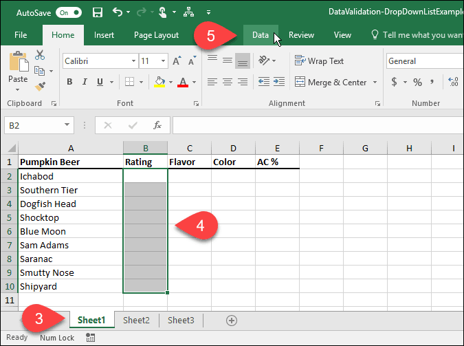
For this example, we want to add drop-down lists to the Rating column or column B. Select the cells you want to add the drop-down lists to. In our case, we selected B2 through B10. Then, click the Data tab.
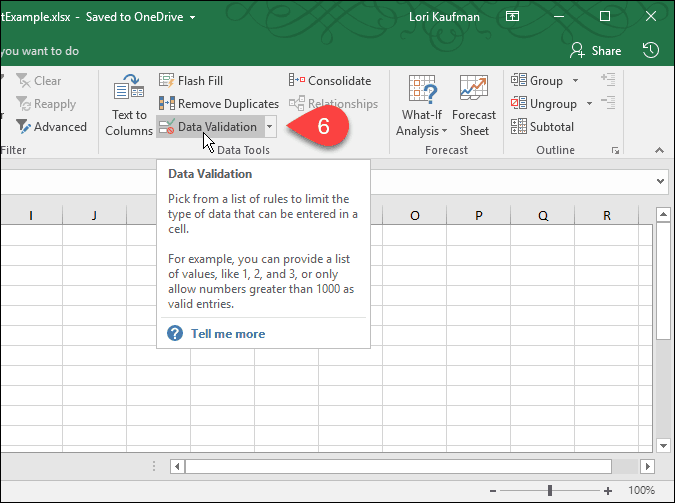
In the Data Tools section, click the Data Validation button.
Add a Drop-Down List to the Selected Cells
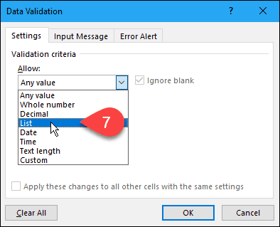
The Data Validation dialog box displays. On the Settings tab, you can have Excel restrict entries in the selected cells to dates, numbers, decimals, times, or a certain length. For our example, select List from the Allow drop-down list to create a drop-down list in each of the selected cells.
Select the Source for the Drop-Down List Options
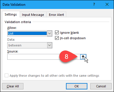
Now, we need to specify the source for the options in each drop-down list. There are two ways you can do this. The first method involves manually typing the options in the Source box separated by commas. This can be time-consuming if you have a long list of items. Earlier in this article, we created a list of items on a separate worksheet. We’re now going to use that list to populate the drop-down list in each of the selected cells. This second method is easy to manage. You can also hide the worksheet containing the options (right-click on the worksheet tab and select Hide) when you distribute the workbook to your users. To add the list from the separate worksheet to your drop-down list, click the up arrow on the right side of the Source box.
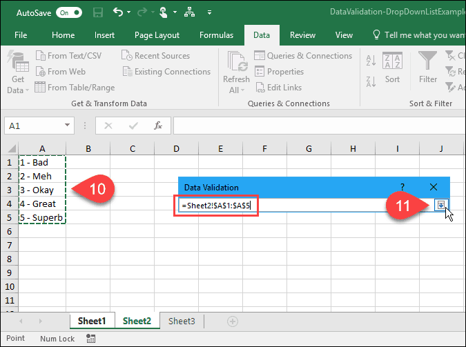
The Data Validation dialog box shrinks down to just the Source box, and you can access your workbook under the dialog box. Click the tab for the worksheet containing the drop-down list options.
Next, select the cells containing the options. The worksheet name and the cell range with the options are added to the Source box on the Data Validation dialog box. Click the down arrow on the right side of the Source box to accept the input and expand the dialog box.
Add an Input Message
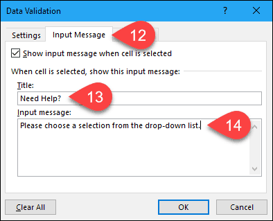
You can add an optional message to the drop-down list. Maybe you want to display a help message or tip. It’s a good idea to keep the message short. To add a message that displays when a cell containing the drop-down list is selected, click the Input Message tab. Next, enter a Title and the Input message in the boxes.
Add an Error Alert
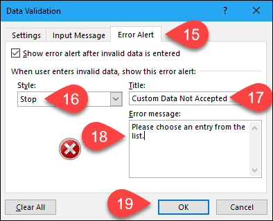
Another option item on the drop-down list is an error message, which would display when a user tried to enter data that doesn’t match the validation settings. In our example, the error message displays when someone types an option into the cell that doesn’t match any of the preset options. To add an error message, click the Error Alert tab. The default option for the Style of the error alert is Stop. You can also select Warning or Information. For this example, accept the default option of Stop in the Style drop-down list. Enter the Title and Error message for the Error Alert. It’s best to keep the error message short and informational. Click OK.
Use Your New Drop-Down List
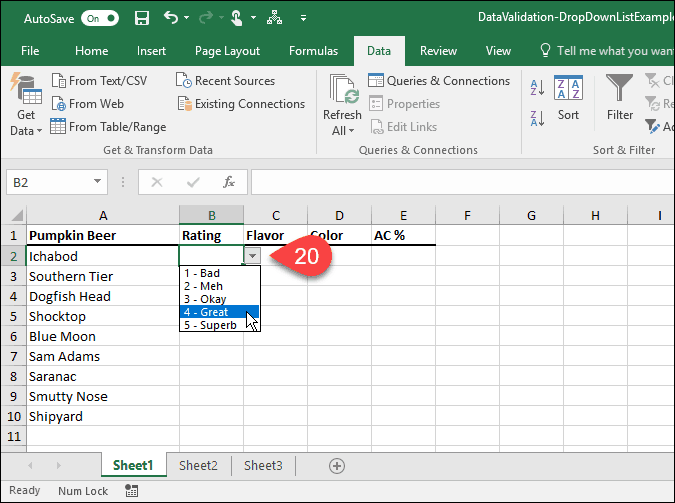
Now, when you click on a cell to which you added a data validation list, a drop-down list will display, and you can select an option.
If you added an Input Message to the drop-down list, it displays when you select a cell containing the drop-down list.
If you try to enter an option that doesn’t match any of the preset options, the Error Alert you set up displays on a dialog box.
How have you made use of drop-down lists in Excel? Let us know in the comments. Also, check out our other Microsoft Office tips and our tutorial for creating drop-downs in Google Sheets. Comment Name * Email *
Δ Save my name and email and send me emails as new comments are made to this post.


![]()
